14. Assessing Read Quality

Questions:

• How can I describe the quality of my data?

Objectives:

• “Explain how a FASTQ file encodes per-base quality scores.”
• “Interpret a FastQC plot summarizing per-base quality across all reads.”
• “Use for loops to automate operations on multiple files.”

Keypoints:

• “Quality encodings vary across sequencing platforms.”
• “for loops let you perform the same set of operations on multiple files with a single command.”

---

15. Starting with Data

Often times, the first step in a bioinformatics workflow is getting the data you want to work with onto a computer where you can work with it. If you have sequenced your own data, the sequencing center will usually provide you with a link that you can use to download your data. Today we will be working with publicly available sequencing data.

About the Dataset: We are studying a population of Escherichia coli (designated Ara-3), which were propagated for more than 50,000 generations in a glucose-limited minimal medium. We will be working with three samples from this experiment, one from 5,000 generations, one from 15,000 generations, and one from 50,000 generations. The population changed substantially during the course of the experiment, and we will be exploring how with our variant calling workflow. The data are paired-end, so we will download two files for each sample. We will use the European Nucleotide Archive to get our data. The ENA provides a comprehensive record of the world’s nucleotide sequencing information, covering raw sequencing data, sequence assembly information and functional annotation.

First, create the project directory and sub-directories:

cd ~/
mkdir -p dc_workshop/data
cd dc_workshop/data

To download the data, run the commands below. It will take about 10 minutes to download the files.

$ cp /opt/dc_workshop/data/*.fastq.gz .

The data comes in a compressed format, which is why there is a .gz at the end of the file names. This makes it faster to transfer, and allows it to take up less space on our computer. Let’s unzip one of the files so that we can look at the fastq format.

$ gunzip SRR2584863_1.fastq.gz

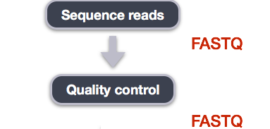
16. Quality Control

We will now assess the quality of the sequence reads contained in our fastq files.

16.1. Details on the FASTQ format

Although it looks complicated (and it is), we can understand the fastq format with a little decoding. Some rules about the format include…

1. Always begins with ‘@’ and then information about the read
2. The actual DNA sequence
3. Always begins with a ‘+’ and sometimes the same info in line 1
4. Has a string of characters which represent the quality scores; must have same number of characters as line 2

• FASTQ Wikipedia

We can view the first complete read in one of the files our dataset by using head to look at the first four lines.

$ head -n 4 SRR2584863_1.fastq

@SRR2584863.1 HWI-ST957:244:H73TDADXX:1:1101:4712:2181/1
>TTCACATCCTGACCATTCAGTTGAGCAAAATAGTTCTTCAGTGCCTGTTTAACCGAGTCACGCAGGGGTTTTTGGGTTACCTGATCCTGAGAGTTAACGGTAGAAACGGTCAGTACGTCAGAATTTACGCGTTGTTCGAACATAGTTCTG
>+
>CCCFFFFFGHHHHJIJJJJIJJJIIJJJJIIIJJGFIIIJEDDFEGGJIFHHJIJJDECCGGEGIIJFHFFFACD:BBBDDACCCCAA@@CA@C>C3>@5(8&>C:9?8+89<4(:83825C(:A#########################

Exercise

What is the last read in the SRR2584863_1.fastq file? How confident are you in this read?

16.2. Assessing Quality using FastQC

In real life, you won’t be assessing the quality of your reads by visually inspecting your FASTQ files. Rather, you’ll be using a software program to assess read quality and filter out poor quality reads. We’ll first use a program called FastQC to visualize the quality of our reads.

FastQC has a number of features which can give you a quick impression of any problems your data may have, so you can take these issues into consideration before moving forward with your analyses. Rather than looking at quality scores for each individual read, FastQC looks at quality collectively across all reads within a sample. The image below shows one FastQC-generated plot that indicates a very high quality sample:

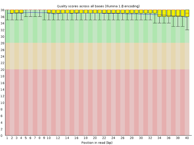
The x-axis displays the base position in the read, and the y-axis shows quality scores. In this example, the sample contains reads that are 40 bp long. This is much shorter than the reads we are working with in our workflow. For each position, there is a box-and-whisker plot showing the distribution of quality scores for all reads at that position. The horizontal red line indicates the median quality score and the yellow box shows the 2nd to 3rd quartile range. This means that 50% of reads have a quality score that falls within the range of the yellow box at that position. The whiskers show the range to the 1st and 4th quartile.

For each position in this sample, the quality values do not drop much lower than 32. This is a high quality score. The plot background is also color-coded to identify good (green), acceptable (yellow), and bad (red) quality scores.

Now let’s take a look at a quality plot on the other end of the spectrum.

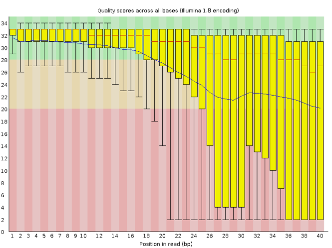
Here, we see positions within the read in which the boxes span a much wider range. Also, quality scores drop quite low into the “bad” range, particularly on the tail end of the reads. The FastQC tool produces several other diagnostic plots to assess sample quality, in addition to the one plotted above.

16.3. Running FastQC

Note: If you haven’t added conda to your PATH yet, please do so by running the following:

echo export PATH=$PATH:/opt/miniconda3/bin >> ~/.bashrc

Then, run the following command (or start a new terminal session) in order to activate the conda environment:

source ~/.bashrc

We will now assess the quality of the reads that we downloaded. First, make sure you’re still in the untrimmed_fastq directory with the pwd command if not, change directory using:

$ cd ~/dc_workshop/untrimmed_fastq/

Exercise

How big are the files? (Hint: Look at the options for the ls command to see how to show file sizes.)

FastQC can accept multiple file names as input, and on both zipped and unzipped files, so we can use the *.fastq* wildcard to run FastQC on all of the FASTQ files in this directory.

$ fastqc *.fastq*

You will see an automatically updating output message telling you the progress of the analysis. It will start like this:

Started analysis of SRR2584863_1.fastq
Approx 5% complete for SRR2584863_1.fastq
Approx 10% complete for SRR2584863_1.fastq
Approx 15% complete for SRR2584863_1.fastq
Approx 20% complete for SRR2584863_1.fastq
Approx 25% complete for SRR2584863_1.fastq
Approx 30% complete for SRR2584863_1.fastq
Approx 35% complete for SRR2584863_1.fastq
Approx 40% complete for SRR2584863_1.fastq
Approx 45% complete for SRR2584863_1.fastq
....
Approx 80% complete for SRR2589044_2.fastq.gz
Approx 85% complete for SRR2589044_2.fastq.gz
Approx 90% complete for SRR2589044_2.fastq.gz
Approx 95% complete for SRR2589044_2.fastq.gz
Analysis complete for SRR2589044_2.fastq.gz
$

For each input FASTQ file, FastQC has created a .zip file and a .html file. The .zip file extension indicates that this is actually a compressed set of multiple output files. We’ll be working with these output files soon. The .html file is a stable web-page displaying the summary report for each of our samples.

We want to keep our data files and our results files separate, so we will move these output files into a new directory within our results/ directory.

$ mkdir -p ~/dc_workshop/results/fastqc_untrimmed_reads
$ mv *.zip ~/dc_workshop/results/fastqc_untrimmed_reads/
$ mv *.html ~/dc_workshop/results/fastqc_untrimmed_reads/

Now we can navigate into this results directory and do some closer inspection of our output files.

$ cd ~/dc_workshop/results/fastqc_untrimmed_reads/

16.3.1. MultiQC

If you would like to aggregate all of your fastqc reports across many samples, MultiQC will do this into a single report for easy comparison.

Run MultiQC:

multiqc .

Note The . which follows the multiqc command is UNIX representation for the current folder.

The terminal output should look like this:

[INFO   ]         multiqc : This is MultiQC v1.7
[INFO   ]         multiqc : Template    : default
[INFO   ]         multiqc : Searching '.'
[INFO   ]          fastqc : Found 8 reports
[INFO   ]         multiqc : Compressing plot data
[INFO   ]         multiqc : Report      : multiqc_report.html
[INFO   ]         multiqc : Data        : multiqc_data
[INFO   ]         multiqc : MultiQC complete

16.4. Viewing the FastQC results

If we were working on our local computers, we’d be able to display each of these HTML files as a webpage:

$ open SRR2584863_1_fastqc.html

However, if you try this on your remote instance, you’ll get an error:

Couldnt get a file descriptor referring to the console

This is because the remote instance we’re using doesn’t have any web browsers installed on it, so the remote computer doesn’t know how to open the file. We want to look at the webpage summary reports, so let’s transfer them to our local computers (i.e. your laptop).

To transfer a file from a remote server to our own machines, we will use scp, which we learned yesterday in the Shell Genomics lesson.

First we will make a new directory on our computer to store the HTML files we’re transfering. Let’s put it on our desktop for now. Open a new tab in your terminal program (you can use the pull down menu at the top of your screen or the Cmd+t keyboard shortcut) and type:

$ mkdir -p ~/Desktop/fastqc_html

Now we can transfer our HTML files to our local computer using scp.

$ scp cyverseusername@ipaddress:/home/sateeshp/dc_workshop/results/fastqc_untrimmed_reads/*.html ~/Desktop/fastqc_html/

• The first part of the command sateeshp@128.196.142.26 is the address for your remote computer.
• The second part starts with a : and then gives the absolute path of the files you want to transfer from your remote computer. Don’t forget the :. We used a wildcard (*.html) to indicate that we want all of the HTML files.
• The third part of the command gives the absolute path of the location you want to put the files. This is on your local computer and is the directory we just created ~/Desktop/fastqc_html.

You should see a status output like this:

SRR097977_fastqc.html                       100%  576KB   1.6MB/s   00:00    
SRR098026_fastqc.html                       100%  620KB   3.3MB/s   00:00    
SRR2584863_1_fastqc.html                    100%  626KB   3.1MB/s   00:00    
SRR2584863_2_fastqc.html                    100%  632KB   3.1MB/s   00:00    
SRR2584866_1_fastqc.html                    100%  631KB   3.2MB/s   00:00    
SRR2584866_2_fastqc.html                    100%  626KB   3.6MB/s   00:00    
SRR2589044_1_fastqc.html                    100%  626KB   3.7MB/s   00:00    
SRR2589044_2_fastqc.html                    100%  627KB   3.1MB/s   00:00    
multiqc_report.html                         100% 1174KB   4.0MB/s   00:00

Exercise

Discuss your results with a neighbor. Which sample(s) looks the best in terms of per base sequence quality? Which sample(s) look the worst?

Solution All of the reads contain usable data, but the quality decreases toward the end of the reads.

16.5. Decoding the other FastQC outputs

We’ve now looked at quite a few “Per base sequence quality” FastQC graphs, but there are nine other graphs that we haven’t talked about! Below we have provided a brief overview of interpretations for each of these plots. It’s important to keep in mind

• Per tile sequence quality: the machines that perform sequencing are divided into tiles. This plot displays patterns in base quality along these tiles. Consistently low scores are often found around the edges, but hot spots can also occur in the middle if an air bubble was introduced at some point during the run.
• Per sequence quality scores: a density plot of quality for all reads at all positions. This plot shows what quality scores are most common.
• Per base sequence content: plots the proportion of each base position over all of the reads. Typically, we expect to see each base roughly 25% of the time at each position, but this often fails at the beginning or end of the read due to quality or adapter content.
• Per sequence GC content: a density plot of average GC content in each of the reads.
• Per base N content: the percent of times that ‘N’ occurs at a position in all reads. If there is an increase at a particular position, this might indicate that something went wrong during sequencing.
• Sequence Length Distribution: the distribution of sequence lengths of all reads in the file. If the data is raw, there is often on sharp peak, however if the reads have been trimmed, there may be a distribution of shorter lengths.
• Sequence Duplication Levels: A distribution of duplicated sequences. In sequencing, we expect most reads to only occur once. If some sequences are occurring more than once, it might indicate enrichment bias (e.g. from PCR). If the samples are high coverage (or RNA-seq or amplicon), this might not be true.
• Overrepresented sequences: A list of sequences that occur more frequently than would be expected by chance.
• Adapter Content: a graph indicating where adapter sequences occur in the reads.